How to Split Text into Multiple Columns in Excel Worksheet?

Sometimes, data from web comes in a way we didn't expect. A bunch of data may be in one column so the data in this worksheet looks like a mess.

We've got some methods to solve this problem. Now, come on with us.

Method 1: Utilize Data Tool to split in Excel.

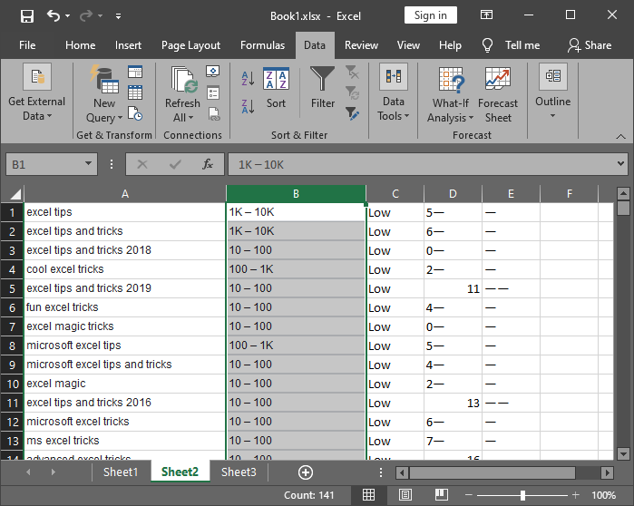
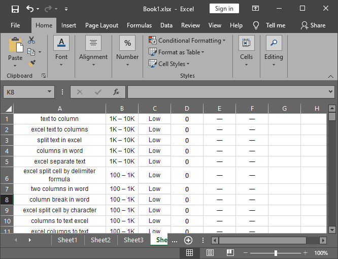
Let's take a look at this worksheet first.

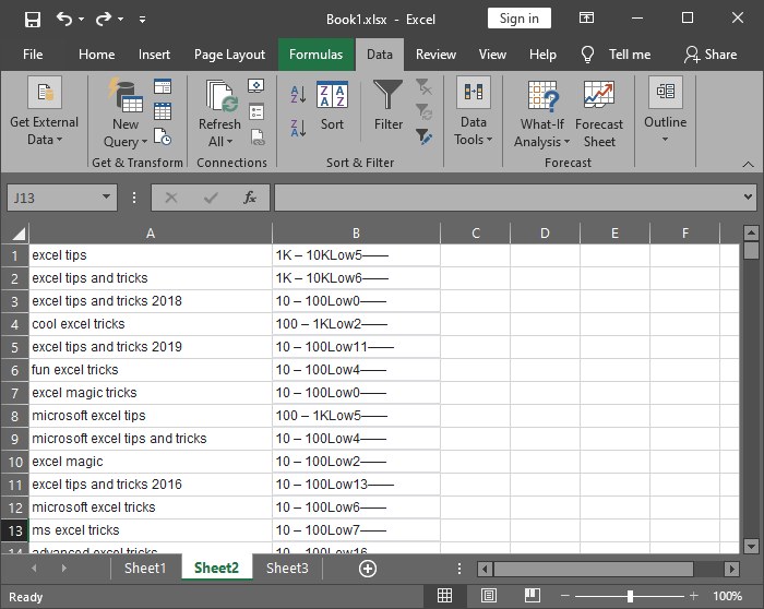
You can tell there are four kinds of data in Column B. Or you couldn't cause it's messed up. Anyway, data in Column B is desperate to split.

Now we're using Data Tool in Excel to split it.

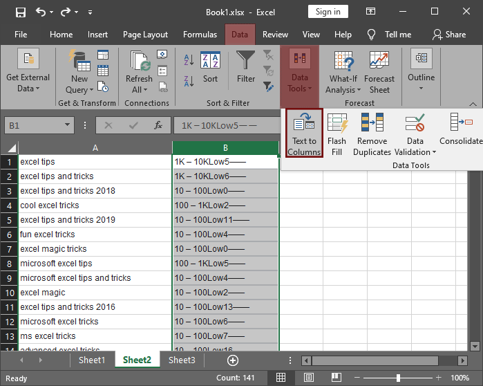
From the outset, select the column need to be separate and then go to Data and choose Data Tools. Select Text to Columns.

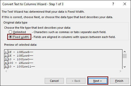
Step 1: Choose Original data type.

Delimited: There are some special characters like commas or tabs could be used as a sign for separate.

Fixed width: Separate the cell based on a fixed width.

Generally, we take advantage of characters such as commas or tabs to separate each field.

But in this case, we don't have any. So, fixed width then.

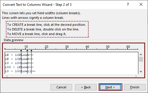
Step 2: Drag and move the line with arrow in Data preview in the bottom.

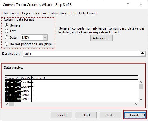
Step 3: Check Data preview and press Finish.

Check the Column data format to make sure it's the data format you want. Or something will wrong. For instance, if it's set as text, you can't launch a formula in this cell.

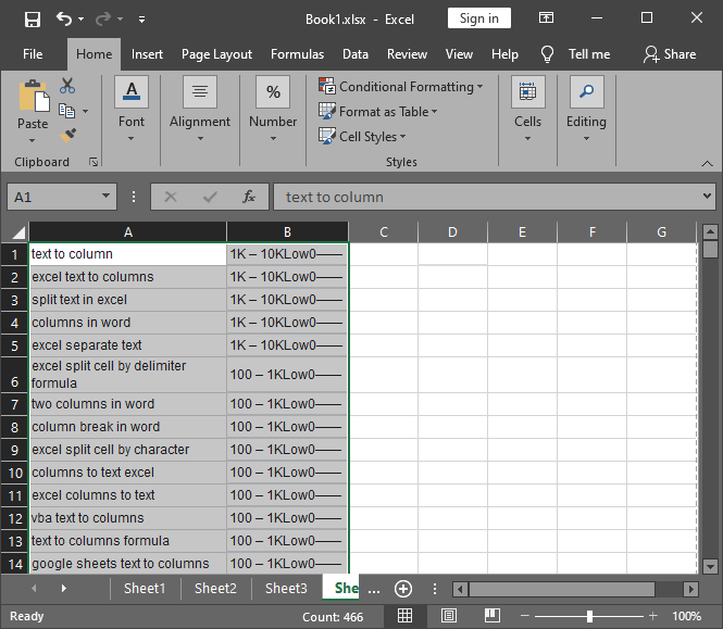
It'll turns out like:

And then make some slight changes on it, it will be neat.

Method 2: Take advantage of functions.

Like what I said, we don't have clear separator characters in the sheet, so, let's try some interesting functions, like these:

LEFT (text, [num_chars])
RIGHT (text, [num_chars])
MID (text, start_num, num_chars)

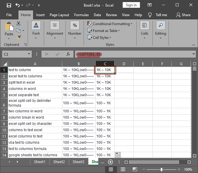
Like the content in Cell B1, I want it to be separated into "1K - 10K", "Low" and "0——".

So, in Cell C1, I input "=LEFT (B1, 8)". This function means that we need the left 8 characters in Cell B1.

Note that a blank space count one.

And drag it down the column, the function will be applied in the left cells.

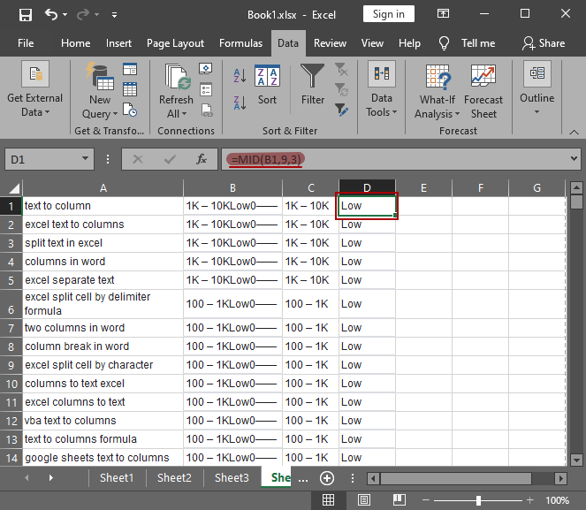
Now we need "Low" in Cell B1 separated, we can use function MID (text, start_num, num_chars).

In this case, I input "=MID (B1, 9, 3)". It means I want the chars in Cell B1 from the 9th character and the following 3.

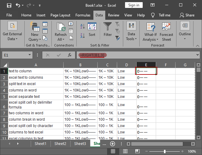
With function RIGHT (text, [num_chars]), we can split out the right characters in the cell.

To do so, I input "=RIGHT (B1, 3)".

I adjust it a bit, finally, it comes out in the way it should be.

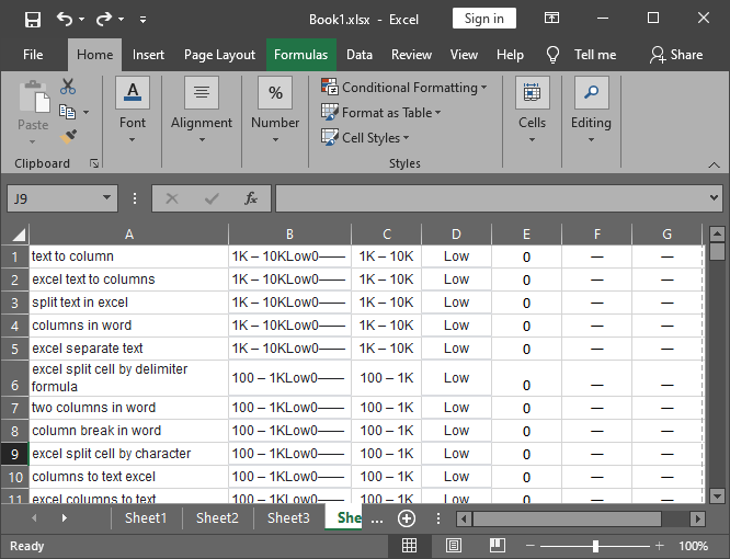
Note: Because these separated data come from data from Column B, if data in Column B is changed or deleted, the separated data will change, too, or worse, it turns out error. To get around this problem, you can follow the process below:

1. Select area from C1 to G20;

2. Copy data in the selected cells and paste data right where it should be, but choose Values in Paste Options;

3. Delete Column B.

Bottom Line:

This article aims at helping people split text in one column into multiple. There are two approaches:

Method 1: Utilize Data Tool to split in Excel.

Method 2: Take advantage of functions for splitting.

Method 1 is easy with only three steps. Method 2 offers three formulas to facilitate people to select almost every part of a cell as they want.

Hope these two methods could help you rearrange your data in Excel worksheet.