How to Filter Data Based on Another List in Excel

The filter function allows us to filter a range of data according to the criteria we define. And it's also useful to filter data based on a list in another worksheet. If there are two worksheets. Sheet1 is a table we need to filter, Sheet2 is a list we base on when filtering data. The question is how to filter the table based on the Sheet2? Read on to discover three methods to filter data based on another list in Excel.

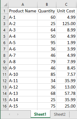
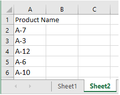
Before filtering data, we need to know how to add filters to a column or a table. Select a cell within the column or table, and select the "Data" tab. Click "Filter" in the Sort & Filter group. Column header arrows will appear in the header of the column or table. There are two worksheets we'll use later. Sheet1 is a table we need to filter, Sheet2 is a list we base on when filtering data. See screenshot.

1. Filter data by using AutoFilter

It's the simplest method to filter data based on another list in Excel. And it's quite suitable for filtering a small amount of data. Check how to filter a small amount of data using AutoFilter below.

a. Add a filter to the table. Select the column header to arrow for the column you want to filter.

b. Uncheck "Select All" and select the item based on the list. Click on the "OK" button. The list will be filtered based on the item in another list.

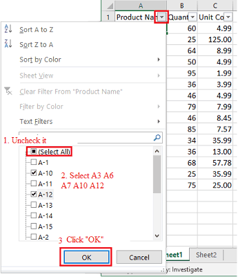
Want to copy and paste the filtered data to another location? Follow the way below.

Select all the filtered data. Click on the Home tab, select "Find & Select" and choose "Go To Special". In the window named "Go to special", choose Visible cells only. Click "OK".

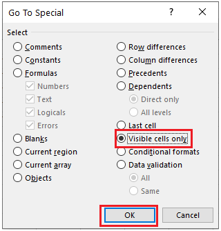
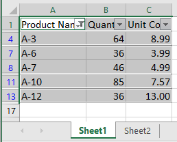
As shown in the picture below, all the extracted data are selected without hidden data. Now the extracted data can be copied and pasted to anywhere you like.

2. Filter data by using the Advanced Filter

Excel's Advanced Filter is more flexible than the basic Excel AutoFilter because it allows users to filter a data range based on user-defined criteria. Therefore, we can regard the list as criteria to filter data easier when we counter a large amount of data. Here's how to filter data using the Advanced Filter.

a. Select a cell in the Sheet1. Click on "Data" in the menu-bar, choose Advanced in the "Sort & Filter" group.

b. In the Advanced Filter dialog box, select the range of table as the List range. Then select the list (including header) as criteria range.

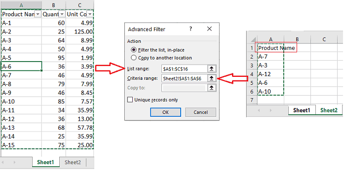
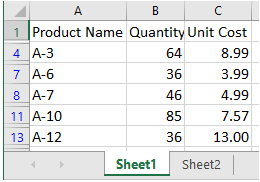
c. Click "OK". The data will be filtered based on Sheet2.

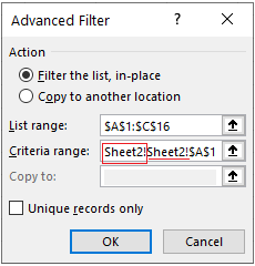
Note: When jumping to another worksheet to select the criteria range, it's easy to have invalid data like a worksheet name. In this situation, delete the redundant information first. Otherwise, an error message that Reference isn't valid will appear. For example, one of the "Sheet2" in the picture below is invalid information and needs to be deleted.

3. Filter data by applying formulas

Applying the COUNTIF formula is quite useful for filtering data based on another list. COUNTIF is a formula to count the number of cells that meet a criterion. When filter data by applying the COUNTIF formula, we need to regard the product name as criteria, data of the list as the range. If the product name is in the list, the result is number 1. If not, the result is 0. Follow this procedure to filter data by applying the COUNTIF formula.

a. Place the cursor to a cell next to the rows you want to filter. Enter the formula below. Then press "Enter" and drag the Autofill handle down to apply this formula to other cells.

=COUNTIF(Sheet2!$A$2:$A$6, Sheet1!A2)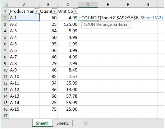

In this formula, "Sheet2!$A$2:$A$6" in the list you want to filter based on. "$" means the range is fixed. You can fix the range by selecting the range and press key F4.

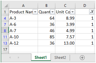
b. Add filter to the formula column. Click the column header arrow for this column and check "1" only.

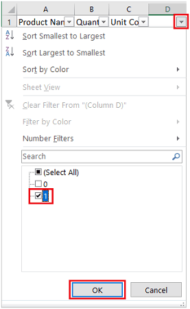
c. Click "OK". Now the rows have been filtered based on the list in Sheet2.

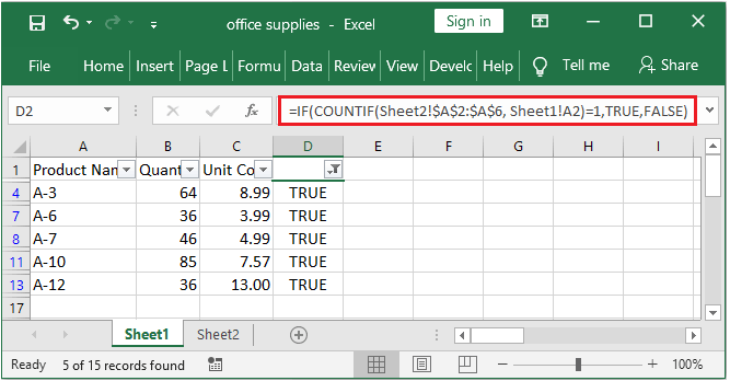
If you want the formula result is True or False, applying the IF and COUNTIF formula. Enter the formula below. If the product name is in the list, the result is TRUE. So after you click the column header arrow for this column, you need to check TRUE only. Click on the "OK" button. Now the rows are been filtered based on another list.

=IF(COUNTIF(Sheet2!$A$2:$A$6, Sheet1!A2)=1,TRUE,FALSE)